Luis DiazSoftware engineer | ||||
| home | blog | projects | about | |
When I was starting to learn how to code I came across donut.c, a program written by Andy Sloane. His goal was to render a donut spinning randomly in a terminal using obfuscated C. Even his code is shaped like a donut:
             k;double sin()
         ,cos();main(){float A=
       0,B=0,i,j,z[1760];char b[
     1760];printf("\x1b[2J");for(;;
  ){memset(b,32,1760);memset(z,0,7040)
  ;for(j=0;6.28>j;j+=0.07)for(i=0;6.28
 >i;i+=0.02){float c=sin(i),d=cos(j),e=
 sin(A),f=sin(j),g=cos(A),h=d+2,D=1/(c*
 h*e+f*g+5),l=cos      (i),m=cos(B),n=s\
in(B),t=c*h*g-f*        e;int x=40+30*D*
(l*h*m-t*n),y=            12+15*D*(l*h*n
+t*m),o=x+80*y,          N=8*((f*e-c*d*g
 )*m-c*d*e-f*g-l        *d*n);if(22>y&&
 y>0&&x>0&&80>x&&D>z[o]){z[o]=D;;;b[o]=
 ".,-~:;=!*#$@"[N>0?N:0];}}/*#****!!-*/
  printf("\x1b[H");for(k=0;1761>k;k++)
   putchar(k%80?b[k]:10);A+=0.04;B+=
     0.02;}}/*****####*******!!=;:~
       ~::==!!!**********!!!==::-
         .,~~;;;========;;;:~-.
             ..,--------,*/
donut.c has a special place in my heart because, the moment I found it, it felt like magic. Now that time has passed and I know much more than I did before, I want to write this article as the explanation I would have liked to have when I saw it for the first time.
One interesting property of donut.c is that it represents the minimally viable version of the graphics rendering pipeline. It develops the basic foundational concepts of a renderer. And the best part is that it can be implemented using a single file, without the need for any additional dependencies beyond the C math library!
In this article, we will step-by-step implement a more readable version of donut.c, this time in C++. Following the spirit of donut.c, we will have the following goals:
torus.cpp.The idea is to create a program that infinitely runs by replacing a character matrix of size $R$ in the terminal with a small variation of itself. However, a terminal is usually intended to print text continuously, leaving a record of the text that has been printed so far, unlike windows where a graphical interface is drawn and updated each iteration of the program. For this reason, the first thing we need to do is find a way to update a set of cells in a terminal instead of continuously stacking them. This varies a bit depending on the terminal emulator you use, but it follows more or less the same pattern in all of them: ANSI escape codes.
ANSI escape codes are used to instruct a terminal emulator to perform a specific action, such as printing characters in a certain color or font or moving the cursor, which is the case we are interested in right now.
We will use ANSI escape codes to instruct the terminal emulator to move the cursor. The cursor is the blinking white bar that marks the position of the next character to be entered. It is usually always at the end of the most recent text, but using ANSI escape codes we can tell it to move to the position we need.
To learn more about ANSI escape codes, you can find a good explanation in this article. For now, we only need to know that the code we need has the following format \033[<some_number>A, where:
\033[ character indicates that we are calling a function.A character is the name of the function, which in this case means “move the cursor up a specific number of rows”.<some_number> character is the argument of the function, which in this case represents the number of rows we want to jump.Now, how can we use this? We want to print and replace a matrix of size $R \times R$, this can be done with the following loop:
// Prints continuously as often as possible
while(true)
{
    // Prints the characters of this line
    for(int i = 0; i < R; i++)
    {
        for(int j = 0; j < R; j++)
        {
            cout << "#";
            // In some terminals, there may be more space between rows than between
            // columns of text. For these cases, we can add a space in the form of
            // padding between columns.
            // cout << " ";
        }
    // Prints the newline character that marks the end of the line
    cout << endl;
  }

  // This is necessary to force the terminal to print what it has in
  // buffer
  cout << flush;
}
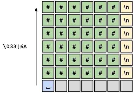
At the end of the double for loop, we will have printed R rows to the terminal, and the cursor will be on row R+1 because the last row also includes a newline character. Moreover, it will be at the beginning of row R+1, so to return to the original position, we only need to move the cursor R rows up, by printing the code \033[RA with cout:
while(true)
{
    // ... nested for loop
    cout << flush;
    cout << "\033[" << R << "A";
}
This is easier to visualize with an example:
Now that we defined a consistent area where we can draw, we still need two things to start working on rendering:
Now, we need to tell the program how often we want it to execute. To do this, we will put our program to sleep for a specified amount of time at the end of each iteration. We need to include thread and chrono. The former gives us access to the function we will use to put our thread to sleep, while the latter allows us to work with time intervals. We can do this by adding the following includes to the beginning of our program:
#include <chrono>
#include <thread>
To put the current thread (the main thread) to sleep, we will use the following line:
this_thread::sleep_for(chrono::milliseconds(30));
this_thread::sleep_for(X) is used to put the main thread to sleep for a specified amount of time.chrono::milliseconds(X) represents an interval of X milliseconds.Later on, we will need a way to know how much time has passed since the start of the application in order to perform operations that depend on that. For this reason, we will also use a variable that stores the time that has elapsed since the start.
// Main loop
auto frame_start = chrono::high_resolution_clock::now();
float time_passed = 0;
while (true)
{
    // Compute the time difference between the start of the previous frame and the current frame,
    // then add it `time_pass`
    auto now = chrono::high_resolution_clock::now();
    auto delta_time = chrono::duration_cast<chrono::milliseconds>(now - frame_start).count() / 1000.0f;
    time_passed += delta_time;
    frame_start = now;

    // ... The rest of the main loop
}
frame_start is an object that represents a point in time. In particular, it represents the start of the frame that is currently being processed.time_passed is the amount of time that has elapsed since the start of the program in secondsnow, and then we calculate the difference in time between now and the last time the loop started, frame_start. We add this difference to time_passed.chrono::duration_cast<chrono::milliseconds>(now - frame_start).count() / 1000.0f; is simply counting the number of milliseconds between now and frame_start, and converting it to seconds.We will now have the amount of time that has passed since the start of the program in time_passed. At the end of each iteration, our program will wait a bit for the next frame.
Right now we are printing the same character continuously in the terminal, but we want the character to depend on the position in the area where we are drawing. We will use a character matrix of size $R \times R$ where we will store the characters that we will draw in the terminal. We will simply create a matrix char canvas[R][R] whose content will be drawn in the terminal:
while(true)
{
    // ... Compute time ...
    for (int i = 0; i < R; i++)
        for (int j = 0; j < R; j++)
            cout << canvas[i][j] << " ";
    // ... The rest of the main loop ...
}
The additional whitespace that is printed after the character is not necessary, but I like the cleaner finish it gives to the resulting image.. If you test the program as it is so far, you may see a matrix of meaningless characters. This is normal, and it is because, depending on where you declared the canvas matrix, its memory may be uninitialized. You can also add a function to clear the canvas before starting, but we will do this later when we update the canvas.
Until now, you should have the following functionality implemented:
Before proceeding, confirm that everything has gone well so far. Then, we will start working on the drawing of our donut.
To update the canvas, our first intuition might be to iterate pixel by pixel over the character matrix, assigning a character to each one depending on its position. This approach is the one we would use with Ray Tracing, but we can do it in a simpler way.
Taking advantage of the low resolution of the terminal, our solution will be a simplification of the computer graphics pipeline. The idea will be as follows:
Before we start, we will set up the function where we will work. The update_canvas function will be responsible for updating the character canvas in each iteration of the main loop. Since our canvas must be accessible to the main function we will pass this matrix by reference to the update function. Thus, the initial version is as follows:
void update_canvas(char (&canvas)[R][R])
{
   // TODO: Actually update canvas
}
The type of the
canvasparameter may seem a bit strange, but the parentheses simply indicate that the parameter is a character matrix passed by reference, instead of an array of character references, which would generate a compilation error. It is important to pass this array by reference because otherwise the entire contents of the array would be copied into the function arguments and this can be a large amount of memory. In addition, the external array would not be modified, so the resulting array would have to be returned by value, which would imply yet another copy.
We will add this function to our main loop, just before printing the characters to the terminal.
while(true)
{
    // ... Compute time ...
    update_canvas(canvas);
    for (int i = 0; i < R; i++)
        for (int j = 0; j < R; j++)
            cout << canvas[i][j] << " ";
    // ... The rest of the main loop ...
}
Now that we have our update_canvas function in place, we can start working on implementing it.
Before we start, we will clean up the canvas by assigning a whitespace character ' ' to each cell, this way it will be “blank”. We need to do this because we will only assign a color to a cell if it corresponds to a torus point. If there’s no torus point for that cell, its content will be unmodified.
void update_canvas(char (&canvas)[R][R])
{
    // Clean up the canvas assigning a
    // whitespace character to each position
   for(int i = 0; i < R; i++)
        for(int j = 0; j < R; j++)
            canvas[i][j] = ' ';
}
The next step is to generate torus points. Normally, we would load a model from a file, but the torus is a parametric shape, and therefore we can use a function to generate the vertices. We will use the following function:
$$ P(\theta, \phi) = \begin{cases} (r_a + r_b\cos(\theta)) \cos(\phi)\ (r_a + r_b\cos(\theta)) \sin(\phi)\ -r_b\cos(\theta) \end{cases} \quad 0\le \theta \le 2\pi,\quad 0\le \phi \le 2\pi $$
Where:
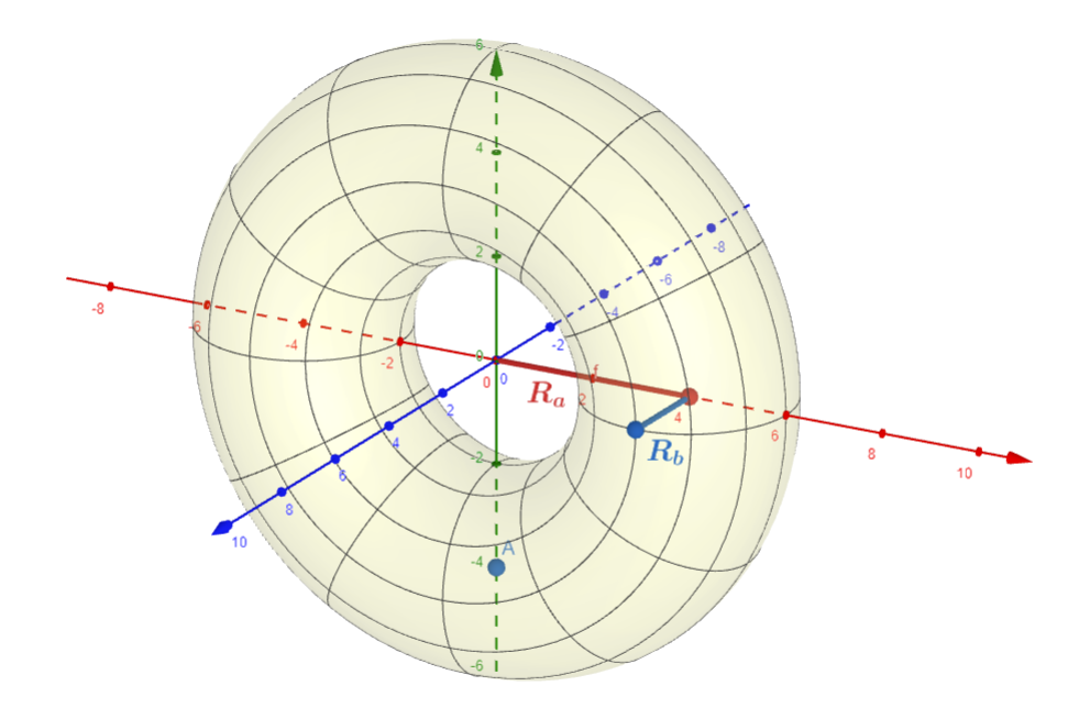
The parameters \( \color{red}{R_a} \), \( \color{blue}{R_b} \) correspond to the radii of the circle and the tube, respectively. The axes are \( \color{red}X \), \( \color{green}Y \), \( \color{blue}Z \).
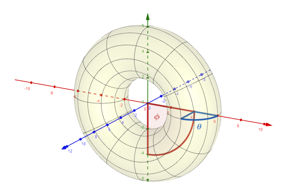
The angle \( \color{blue}{\theta} \) corresponds to the angle on the circumference of the tube, and the angle \( \color{red}{\phi} \) corresponds to the angle on the inner circumference.
To represent this parametric equation for a torus, we will use the following function:
void torus_point(float theta, float phi, float torus_radius, float tube_radius, float &out_x, float &out_y, float &out_z)
{
    out_x = (torus_radius + tube_radius * cos(theta)) * cos(phi);
    out_y = (torus_radius + tube_radius * cos(theta)) * sin(phi);
    out_z = -tube_radius * sin(theta);
}
To use cos and sin we will need to include math, with #include <math>.
This function computes the three coordinates of a torus point using the equation we showed earlier. Note that, since we will return three values, the variables where the results are stored are passed by reference. As an additional exercise, you could implement a struct that represents a point or vector. In this article, we won’t do this to limit ourselves to variables, functions, and basic control structures.
The torus is a continuous surface, which means that it has infinite points, but we only need a few.
Since we have two values that parameterize the torus’ surface, $\color{blue} \theta, \color{red} \phi$, then to get a set of vertices we need a sequence of pairs of values for $\color{blue} \theta, \color{red} \phi$. To choose these pairs, we will iterate over the rings and vertices per ring, similar to how we would iterate over a matrix.
To know how many pairs of values we will generate we need to choose a resolution. The resolution tells us how many rings and vertices per ring we will have. The higher the resolution of the model, the higher the quality of the resulting model will be, but it will also take up more memory and processing time. In our case, since the terminal has a very low resolution, we don’t need a very detailed model. For simplicity, we will use the same resolution for the number of rings and vertices.
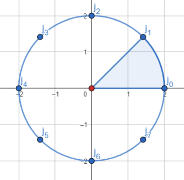
This is one of the rings of the torus, it can be seen as a cut in the torus tube. Each point corresponds to a vertex on the surface of the torus. Since the resolution is 8, we have 8 vertices per ring.
Note that since $0 \leq {\color{blue}\theta}, {\color{red}\phi} \leq 2 \pi$, then the angle between each pair of points is $2\pi / resolution$.
Finally, we can compute the vertices we need with the following function:
void update_canvas(char (&canvas)[R][R])
{
    // ... Clear the canvas ...
    const int TORUS_RESOLUTION = 200; // Choose a resolution
    // The angle between each adjacent pair of rings or vertices.
    // M_PI comes from `math`
    const float step_size = (2.f * M_PI) / TORUS_RESOLUTION;

    // Compute each radius in the torus. In this case I will base
    // the radius in the canvas resoution.
    const float tube_radius = ((float) R) / 4.f;
    const float torus_radius = ((float) R) / 2.f;

    for (int i = 0; i < TORUS_RESOLUTION; i++)
    {
        const float phi = step_size * i;
        for (int j = 0; j < TORUS_RESOLUTION; j++)
        {
            const float theta = step_size * j;
            float x, y, z; // Vertex coordinates
            torus_point(theta, phi,torus_radius, tube_radius, x, y, z);
        }
    }
}
As we mentioned at the beginning, we will use a vertex-oriented approach, so we will iterate over the vertices of the model instead of the pixels of the image. For this reason, most of the work will be focused on this loop that we just created.
At this point, we can update the canvas and generate vertices for the torus surface. However, we still don’t see anything in the terminal. We will add some temporary code that will help us to have better feedback on our work.
void update_canvas(char (&canvas)[R][R])
{
    // ... Clear the canvas ...
    // ... Choose each torus radius and resolution ...

      for (int i = 0; i < TORUS_RESOLUTION; i++)
      {
        const float phi = step_size * i;
        for (int j = 0; j < TORUS_RESOLUTION; j++)
        {
            const float theta = step_size * j;
            // ... Compute x,y,z position of the current vertex ...
            int x_int, y_int;
            x_int = (int) x;
            y_int = (int) y;
            if (0 <= x_int && x_int < R && 0 <= y_int && y_int < R)
            {
                canvas[y_int][x_int] = '#';
            }
        }
    }
}
# if it contains a vertex.The following image shows the relationship between the canvas and the torus geometry. The position [0][0] of the matrix corresponds to the points in the interval $[0,1)\times[0,1)$, the slot [0][1] to the points in $[0,1)\times[1,2)$, and so on. In other words, the canvas is a window that goes from the origin to the point $(R, R)$.
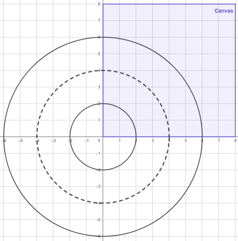
Note that the Y-axis is reflected downwards in our canvas, since the row indices increase downwards, while in the Cartesian plane, they increase upwards. In other words, the positive Y-axis points downwards, just like in Godot. For this reason, the image you will see at this point will be the torus arc in the first quadrant of the plane but reflected across the X-axis.
Although we can visualize the torus in the terminal, it is possible that we cannot see it completely or that it is incorrectly located in the image. For this reason, we will add transformation functions below to be able to see the torus.
We will add the following translation function:
void translate(float offset_x, float offset_y, float offset_z, float x, float y, float z, float& out_x, float& out_y, float& out_z)
{
    out_x = x + offset_x;
    out_y = y + offset_y;
    out_z = z + offset_z;
}
This function simply takes the original coordinates and adds a displacement. We can use it to move the torus vertices on the canvas.
We will also add the scaling function since the torus may be too large to be visible on the canvas.
void scale(float scale, float x, float y, float z, float& out_x, float& out_y, float& out_z)
{
    out_x = scale * x;
    out_y = scale * y;
    out_z = scale * z;
}
The scaling function is useful for testing purposes, but later we will use perspective projection to scale the torus by modifying its distance to the camera. For now, scaling will help us to see the torus.
With the following code, just after creating the torus vertices, we can center the torus on our canvas:
// Update Canvas:
    // ... Clear Canvas ...
    // ... Choose radius and resolution ...

    for (int i = 0; i < TORUS_RESOLUTION; i++)
    {
        const float phi = step_size * i;
        for (int j = 0; j < TORUS_RESOLUTION; j++)
        {
            const float theta = step_size * j;
            // ... Compute x,y,z positon of the actual vertex ...
            scale(0.5, x,y,z, x,y,z);
            translate(R / 2, R / 2, 40, x,y,z, x,y,z);
            // ... Assign # to the matrix position that contains this vertex ...
        }
    }
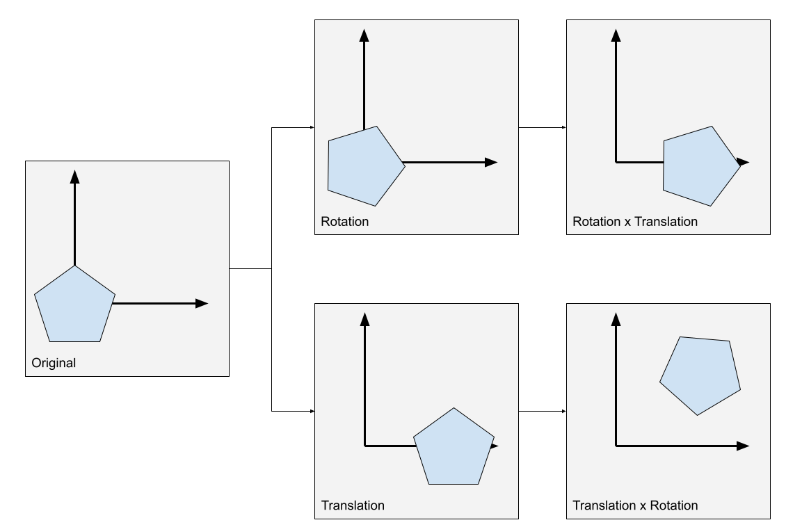
📝 Note: It is possible to rotate after translating, using the rotation matrix that also depends on the rotation axis. The rotation matrices we are using assume that the rotation axis is at the origin (each axis of the origin depending on the rotation), and we will stick with them for simplicity.
Projection is the process of transforming a 3D geometric representation into a 2D one. In our case, we want to transform 3D points into a 2D image. To get a projection we just need a function that transforms 3D points into 2D points.
Currently, we are using orthographic projection. That is, we convert points $(x,y,z)$ into points $(x’, y’)$ simply by discarding the Z coordinate:
$$ Ortho(x,y,z) = (x,y) $$
This projection type is the one we have being using so far, is simple and allows us to visualize 3D objects easily. However, it does not consider depth, so objects that are far away look the same size as if they were closer. Intuitively, this is a consequence of ignoring the Z coordinate. Our projection function ignores the depth of vertices.
.png)
Orthographic Projection: Vertices inside the cube are projected into the plane by discarding their Z coordinate.
Now we will implement perspective projection, a style of projection that takes depth into account so that distant objects appear smaller than objects close to the camera. The idea is to scale the points $(x,y)$ linearly with respect to their $z$ coordinate. For this, let’s consider the following image:
.png)
The idea is to create a virtual 2D plane that is at a certain distance from the camera and project the vertices of our 3D geometry onto this 2D surface. The content of the plane will be drawn to the canvas. To achieve this transformation, we will consider the theorem of triangle proportionality, or Thales’s theorem to determine the position $(x’, y’)$ in this virtual plane.
Thales’s theorem tells us that if we intersect a triangle with a line parallel to one of its sides, we obtain the following relationships:
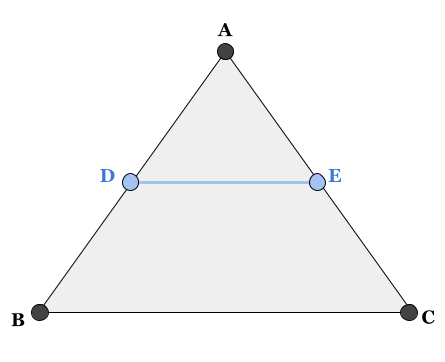
$$ \textbf{(a)} \frac{|AD|}{|DB|} = \frac{|AE|}{|EC|} \ \textbf{(b)} \frac{|AD|}{|AB|} = \frac{|AE|}{|AC|} = \frac{|DE|}{|BC|} $$
In this example, the line segment $\color{blue}{DE}$ is parallel to $BC$, and the intersection points will introduce these relationships. As we will see later, the most useful relationship will be $(b)$, since it will allow us to relate the length of the intersection line $\color{blue}{DE}$ with the length of the line segments it intersects.
Now let’s see with more detail the definition of our virtual plane to identify where to use the Thales theorem:
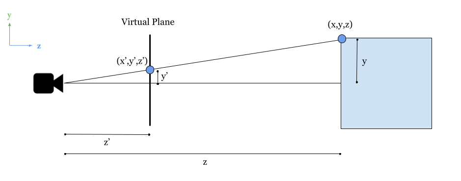
In this image, we see a lateral perspective of the camera. Assuming that it is located at the origin, we can identify the following values:
Using part (b) of Thales’s theorem, we can derive the following relationship:
$$ \frac{z}{z’} = \frac{y}{y’} $$
And since the only unknown value is $y’$, then we can solve the equation for $y’$:
$$ y’ = \frac{y z’}{z} $$
Similarly, we can use the same logic to find the value of $x’$:
$$ x’=\frac{xz’}{z} $$
To find such a value we can consider the projection in the $XZ$ plane instead of the $YZ$ that we used in the previous image. This projection corresponds to a top-down camera view.
Finally, our perspective projection function is:
$$ Perspective(x,y,z) = (\frac{xz’}{z}, \frac{yz’}{z}) $$
Where:
Now, taking our newly acquired theory to our program, we will return to the canvas update function, specifically to the part where we project 3D points to 2D points:
    // Update Canvas:
    // ... Clear canvas ...
    // ... Choose torus radius and resolution ...

    for (int i = 0; i < TORUS_RESOLUTION; i++)
    {
        const float phi = step_size * i;
        for (int j = 0; j < TORUS_RESOLUTION; j++)
        {
            const float theta = step_size * j;
            // ... Compute the x,y,z position of the current vertex ...
            // ... Compute rotations, translations and scale ...
            int x_int, y_int;
            // Replace orthographic projection....
            // x_int = (int) x;
            // y_int = (int) y;
            // with perspective projection:
            x_int = (int) (CAM_DISTANCE_TO_SCREEN * x / z);
            y_int = (int) (CAM_DISTANCE_TO_SCREEN * y / z);
            if (0 <= x_int && x_int < R && 0 <= y_int && y_int < R)
            {
                canvas[y_int][x_int] = '#';
            }
        }
    }
CAM_DISTANCE_TO_SCREEN is a constant float that represents $z’$ in our previous equation. You can define it anywhere in the program as long as it is accessible at this point. In my case, I will use the value of 20.0.scale(0.5, x,y,z, x,y,z);Now that we have perspective projection, the parts of the torus that are farthest from the camera should appear smaller than the parts that are closest to the camera. At this point, we only need to color the torus so that each point on its surface has a different color depending on its angle with respect to the light.
Shading is simply choosing a color for each pixel of the image. We will not use real colors, but rather ASCII characters. In our case, the problem is reduced to finding the correct character for each “pixel”. We will use denser characters according to the “brightness” of the color at each point. The characters we will use, ordered from darker to lighter, are:
.,-~:;=!*#$@
To define the brightness of each point, we will use a very simple rule. We will choose a direction of light, and depending on the angle of the normal at each point on the surface to this direction, we will consider that this point is brighter.
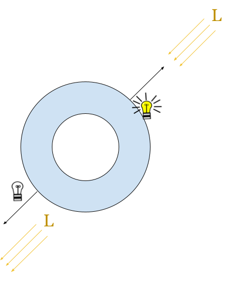
To achieve this we will use the dot product between the direction of light and the surface’s normal vector. As we know, the dot product is a function that takes two vectors and calculates a scalar value. When the vectors are normalized, then the scalar is in the range \( [-1,1] \), where -1 indicates that they are antiparallel (they are the same vector with opposite directions) and 1 indicates that they are parallel (they are the same vector, including the direction), and 0 indicates that they are perpendicular.
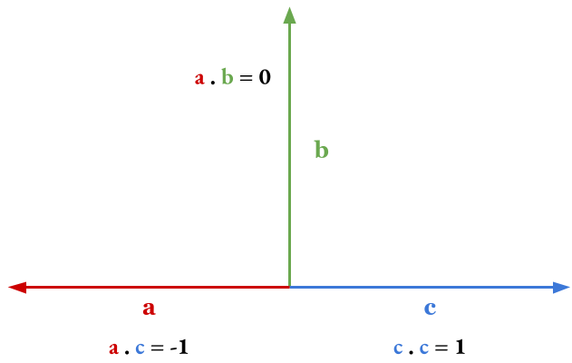
Examples of dot product: $\color{red}a$ and $\color{green}b$ are perpendicular, so their dot product is 0. $\color{red}a$ and $\color{blue}c$ are antiparallel, so their dot product is -1, and $\color{blue}c$ is parallel to itself, so the product with itself is 1. Additionally, all vectors between $\color{blue}c$ and $\color{green}b$ multiplied with $\color{red}a$ return negative values, and all vectors between $\color{blue}c$ and $\color{green}b$ multiplied with $\color{blue}c$ return positive values.
Now that we have an idea about how to color our pixels with characters, we need a plan to make it happen. The following steps are:
A problem we haven’t solved so far is the drawing order. We have been drawing each vertex independently of whether there is another vertex closer to the camera. To solve this, we will use z-buffering. We will create a matrix of the same size as the canvas, which we will call the z-buffer. This matrix will store the distance of the closest vertex drawn at each position on the canvas. If the new vertex we are about to draw is further away than the current vertex in the z-buffer, then we will ignore it.
Now that we have a plan, let’s get to work. We will start by writing the function to compute the torus normal:
Note that the torus is a solid of revolution, a circle translated from the origin and then rotated around it. We know that the normal in any point of a circle is parallel to the vector that comes from the center to that point:
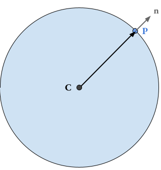
As we can see in this case, the circle with center $C$ has normal $\color{gray}{n}$ at the point $\color{blue} P$, and furthermore $\color{gray}{n}$ is parallel to the vector $C\color{blue} P$. We can extrapolate this same logic to the torus by noticing that each ring of the torus is a circle. The point on the surface of the torus is a point on the circle that we already know how to calculate, so we only need the point at the center of the ring to calculate the normal vector to the surface.
If we recall the torus geometry, we notice that we can compute a vertex in the middle of the tube as a torus with tube radius 0:
In this example, if we force $\color{blue}{R_b} = 0$, then the point we get will be always in the middle of the tube. With this knowledge, we can write the following function:
void torus_normal(float theta, float phi, float torus_radius, float tube_radius, float &out_x, float &out_y, float &out_z)
{
    float p_x, p_y, p_z;
    float c_x, c_y, c_z;

    // Compute a surface point
    torus_point(theta, phi, torus_radius, tube_radius, p_x, p_y, p_z);

    // Compute a point in the center, is the same function as before but
    // with a tube radius == 0
    torus_point(theta, phi, torus_radius, 0, c_x, c_y, c_z);

    // Compute the normal vector as the difference between the center point and the surface vertex:
    out_x = p_x - c_x;
    out_y = p_y - c_y;
    out_z = p_z - c_z;

    // And we normalize the normal vector.
    out_x = out_x / tube_radius;
    out_y = out_y / tube_radius;
    out_z = out_z / tube_radius;
}
torus_point function we defined earlier.With this function, we can now compute the normal at each point in the torus surface using the same parameters we used to compute the vertex.
Now we will create a function to compute the dot product between two vectors, it’s really simple:
float dot(float x1, float y1, float z1, float x2, float y2, float z2)
{
    return x1 * x2 + y1 * y2 + z1 * z2;
}
Now we will define the variables in the update_canvas function for the coordinates of the directional light vector:
    float LIGHT_DIR_X = 0, LIGHT_DIR_Y = 1, LIGHT_DIR_Z = 1;
    float magnitude = sqrt(LIGHT_DIR_X * LIGHT_DIR_X + LIGHT_DIR_Y * LIGHT_DIR_Y + LIGHT_DIR_Z * LIGHT_DIR_Y);
    LIGHT_DIR_X = LIGHT_DIR_X / magnitude;
    LIGHT_DIR_Y = LIGHT_DIR_Y / magnitude;
    LIGHT_DIR_Z = LIGHT_DIR_Z / magnitude;
With these variables, we define the direction of the light, which is on the $y$ axis and points downwards and forwards. Note that it is important to normalize this vector so that our next calculations are accurate.
Before using the normal vector, we need to transform it so that it is consistent with the transformations we have applied to the torus.
The mathematics required to transform normal vectors is a bit beyond the scope of this article, but for now, it is enough to know that in this case we will only need to apply the same rotations that were applied to the point in the same order:
// Update Canvas:
    // ... Clear the canvas ...
    // ... Choose torus radius and resolution ...

    for (int i = 0; i < TORUS_RESOLUTION; i++)
    {
        const float phi = step_size * i;
        for (int j = 0; j < TORUS_RESOLUTION; j++)
        {
            const float theta = step_size * j;
            // ... Compute x,y,z position of the current vertex ...
            // ... Compute rotations, translations and scale ...
            float n_x, n_y, n_z;
            torus_normal(theta, phi,torus_radius, tube_radius, n_x, n_y, n_z);
            rotate_y(time_passed, n_x,n_y,n_z, n_x,n_y,n_z);
            rotate_x(time_passed * 1.13, n_x,n_y,n_z, n_x,n_y,n_z);
            rotate_z(time_passed * 1.74, n_x,n_y,n_z, n_x,n_y,n_z);
            // ... Project this vertex and assign # to its positon in the canvas ...
        }
    }
Finally, let’s assign the right color to each pixel:
// Update Canvas:
    // ... Clear the canvas ...
    // ... Choose torus radius and resolution ...

    for (int i = 0; i < TORUS_RESOLUTION; i++)
    {
        const float phi = step_size * i;
        for (int j = 0; j < TORUS_RESOLUTION; j++)
        {
            const float theta = step_size * j;
            // ... Compute x,y,z position of the current vertex ...
            // ... Compute rotations, translations and scale ...
            // ... Normal transformations ...
            // ... Project this vertex and assign # to its positon in the canvas  ...
            if (0 <= x_int && x_int < R && 0 <= y_int && y_int < R)
            {
                char const SHADES[] = ".,-~:;=!*#$@";
                float normal_dot_light = dot(n_x,n_y,n_z, LIGHT_DIR_X, LIGHT_DIR_Y, LIGHT_DIR_Z);

                // Sanity check
                if (abs(normal_dot_light) >= 1.0f)
                    normal_dot_light = 1.0f;

                // Replace this line ...
                // canvas[y_int][x_int] = '#';
                // With this conditional assign:
                if(normal_dot_light >= 0)
                    canvas[y_int][x_int] = ' ';
                else
                    canvas[y_int][x_int] = SHADES[(int) (abs(normal_dot_light) * 12)];
            }
        }
    }
At this point, it is possible that the image you see does not have the correct colors. This is because we are not checking if we are drawing over a pixel that is already the closest to the screen. To do this, we will use a z-buffer. It’s a matrix of the same size as our canvas where we store the Z component of the point that we have drawn in each pixel. We only draw vertices if the pixel it is assigned is empty or has a point that is further in the 3D space.
// Update Canvas:
    // ... Clear the canvas ...
    // ... Choose torus radius and resolution ...
    float depth_buffer[R][R];
    for(int i = 0; i < R; i++)
        for(int j = 0; j < R; j++)
            depth_buffer[i][j] = 1000000;
    // ... Processing of each torus point ...
Finally, to use the z-buffer we simply check that the point we are about to draw is nearer than the last point that was assigned to the same pixel, and if it is, we have to update the Z buffer:
// Update Canvas:
    // ... Clear the canvas ...
    // ... Choose torus radius and resolution ...

    for (int i = 0; i < TORUS_RESOLUTION; i++)
    {
        const float phi = step_size * i;
        for (int j = 0; j < TORUS_RESOLUTION; j++)
        {
            const float theta = step_size * j;
            // ... Compute x,y,z position of the current vertex ...
            // ... Compute rotations, translations and scale ...
            // ... Normal transformations ...
            // ... Project this vertex and assign # to its positon in the canvas  ...
            // We add a new condition to the if statement:
            if (0 <= x_int && x_int < R && 0 <= y_int && y_int < R && depth_buffer[y_int][x_int] > z)
            {
                depth_buffer[y_int][x_int] = z;
                // ... We chose a color for this pixel ...
            }
        }
    }
And with this, we have finished our program. This was a long journey, but along the way, we learned the basics of computer graphics, and we managed to implement the rendering of a 3D geometric figure using only basic control structures. With this program as a base, it is easier to extend the theory to understand rendering with graphical APIs, such as OpenGL.
With a little more work, it is possible to extend this simple scheme to create more complex rendering styles. You could add a 3D model parser to read the vertices of a 3D along with their normals to create a terminal render that works for any type of 3D geometry instead of just toroids. Going a little further, we could map RGB colors to some ANSI color codes and use UVs to create a simple color rendering. We could even turn it into a recursive Ray Tracer by changing the point-by-point approach we use to a pixel-by-pixel approach, the sky is the limit!
The resulting code of this article can be found in the following Github repo:
GitHub - LDiazN/torus.cpp: A simple torus render in terminal inspired by donut.c